Bioinformatics workflows with snakemake and conda#
Author: Sarah Peter
In this tutorial you will learn how to run a ChIP-seq analysis with the snakemake workflow engine.
Disclaimer: In order to keep this tutorial simple, we use default parameters for the different tools as much as possible. However, for a real analysis you should always adapt the parameters to your dataset. Also, be aware that the results of some steps might be skewed, because we only work on data from one chromosome.
Table of contents#
- Install conda
- Setup the environment
- Working with conda environments
- Create snakemake workflows
- Inspect results in IGV
- Exercises
- (Optional) Revert the changes to your environment
- Useful stuff
- References
- Acknowledgements
Install conda#
For this tutorial we will use the conda package manager to install the required tools.
Conda is an open source package management system and environment management system that runs on Windows, macOS and Linux. Conda quickly installs, runs and updates packages and their dependencies. Conda easily creates, saves, loads and switches between environments on your local computer. It was created for Python programs, but it can package and distribute software for any language.
Conda as a package manager helps you find and install packages. If you need a package that requires a different version of Python, you do not need to switch to a different environment manager, because conda is also an environment manager. With just a few commands, you can set up a totally separate environment to run that different version of Python, while continuing to run your usual version of Python in your normal environment.
It can encapsulate software and packages in environments, so you can have multiple different versions of a software installed at the same time and avoid incompatibilities between different tools. It also has functionality to easily port and replicate environments, which is important to ensure reproducibility of analyses.
Attention when dealing with sensitive data: Everyone can very easily contribute installation recipies to the bioconda channel, without verified identity or double-checking from the community. Therefore it’s possible to insert malicious software. If you use bioconda when processing sensitive data, you should check the recipes to verify that they install software from the official sources.
We will use conda on two levels in this tutorial. First we use a conda environment to install and run snakemake. Second, inside the snakemake workflow we will define separate conda environments for each step.
Set up VirtualBox#
Independent of the operating system you are using, we recommend you set up a VirtualBox as described in our instructions. This ensures that the conda installation does not affect your local environment and all steps in the tutorial work as expected.
In case you still wish to install conda natively on your machine at your own risk, you can check these installation instructions.
Install conda in the VirtualBox VM#
Start the VM in VirtualBox.
Start the
Powershell(Windows) or other terminal application (MacOS, Linux).Connect to the VM with
ssh -p 2222 tutorial@127.0.0.1Password is
lcsblcsbif you have not changed it.
Once connected to the VM, follow these steps to install conda:
$ wget https://repo.anaconda.com/miniconda/Miniconda3-latest-Linux-x86_64.sh
$ chmod u+x Miniconda3-latest-Linux-x86_64.sh
$ ./Miniconda3-latest-Linux-x86_64.sh
You need to specify your installation destination, e.g. /home/tutorial/tools/miniconda3. You must use the full path and cannot use $HOME/tools/miniconda3. Answer yes to initialize Miniconda3.
The installation will modify your .bashrc to make conda directly available after each login. To activate the changes now, run
$ source ~/.bashrcSetup the environment#
Update conda to the latest version:
$ conda update condaIn recent versions the conda update sometimes messes up the permissions of some conda executables. To fix the problem, run
$ chmod +x $(which conda)
$ chmod +x $(which conda-env)
Create a new conda environment and activate it:
$ conda create -n bioinfo_tutorial
$ conda activate bioinfo_tutorial
After validation of the creation step and once activated, you can see that your prompt will now be prefixed with
(bioinfo_tutorial)to show which environment is active. For the rest of the tutorial make sure that you always have this environment active.Make sure Python does not pick up packages in your home directory:
(bioinfo_tutorial) $ export PYTHONNOUSERSITE=TrueInstall snakemake and mamba:
(bioinfo_tutorial) $ conda install -c bioconda -c conda-forge snakemake-minimal mamba
Working with conda environments#
You can list the packages installed in your current environment with:
(bioinfo_tutorial) $ conda listYou can export your current environment to a yaml file with:
(bioinfo_tutorial) $ conda env export > environment.yaml
(bioinfo_tutorial) $ cat environment.yaml
This file can be shared or uploaded to a repository, to allow other people to recreate the same environment.
It contains three main items:
nameof the environment- a list of
channels(repositories) from which to install the packages - a list of
dependencies, the packages to install and optionally their version
When creating this environment file via export, it will list the packages you installed and also all their dependencies and the dependencies of their dependencies down to the lowest level. However, when manually creating the file, it’s sufficient to specify the top-level required packages or tools. All the dependencies will be installed automatically.
For our environment with snakemake, the most simple definition - if we do not care about versions - would be:
name: bioinfo_tutorial
channels:
  - bioconda
  - conda-forge
dependencies:
  - snakemake-minimal
  - mamba
For reproducibility, it is advisable to always specify the version, though.
name: bioinfo_tutorial
channels:
  - bioconda
  - conda-forge
dependencies:
  - snakemake-minimal=6.4.1
  - mamba=0.14.0
Let us deactivate the snakemake environment, delete it and recreate it from the yaml file. You may use the exported yaml or create a minimal one like shown above and use this one.
(bioinfo_tutorial) $ conda deactivate
(base) $ conda remove --name bioinfo_tutorial --all
(base) $ conda env create -f environment.yaml
(base) $ conda activate bioinfo_tutorial
You can list available conda environments with:
(bioinfo_tutorial) $ conda env listYou may want to run this again after the tutorial to see all the environments we created.
Create snakemake workflows#
The Snakemake workflow management system is a tool to create reproducible and scalable data analyses. Workflows are described via a human readable, Python based language. They can be seamlessly scaled to server, cluster, grid and cloud environments, without the need to modify the workflow definition. Finally, Snakemake workflows can entail a description of required software, which will be automatically deployed to any execution environment.
Snakemake is a very useful tool if you need to combine multiple steps using different software into a coherent workflow. It comes with many features desired for running workflows, like
- ensuring all input and result files are present
- restarting at a failed step
- rerunning (parts of a) pipeline when (some of) the input changed
- support for wildcards to apply a step to a set of files
- automatically parallelising where possible
- software management
- collecting benchmark data
- modularisation
- creating launcher scripts and submitting jobs to the cluster
- creating a visualisation of the workflow steps (see below)
In this tutorial we will analyse ChIP-seq data from the paper Gérard D, Schmidt F, Ginolhac A, Schmitz M, Halder R, Ebert P, Schulz MH, Sauter T, Sinkkonen L. Temporal enhancer profiling of parallel lineages identifies AHR and GLIS1 as regulators of mesenchymal multipotency. Nucleic Acids Research, Volume 47, Issue 3, 20 February 2019, Pages 1141–1163, https://doi.org/10.1093/nar/gky1240 published by our colleagues at LSRU.
We will set up the following workflow:

To speed up computing time we use source files that only contain sequencing reads that map to chromosome 12. The files for input (control) and H3K4me3 (ChIP) are available on our WebDAV server.
Create a working directory and download the necessary data:
$ mkdir bioinfo_tutorial
$ cd bioinfo_tutorial
$ curl https://webdav-r3lab.uni.lu/public/biocore/snakemake_tutorial/snakemake_tutorial_data.tar.gz.gpg -o snakemake_tutorial_data.tar.gz.gpg
$ curl https://webdav-r3lab.uni.lu/public/biocore/snakemake_tutorial/snakemake_tutorial_data.tar.gz.gpg.md5 -o snakemake_tutorial_data.tar.gz.gpg.md5
Check the md5 sum:
$ md5sum -c snakemake_tutorial_data.tar.gz.gpg.md5
snakemake_tutorial_data.tar.gz.gpg: OK
Make sure it says OK.
Then decrypt the data with gpg and finally unpack it. The passkey or passphrase for decryption is elixirLU. In real situations the passphrase should always be transmitted in a secure way and separate from the data!
$ gpg -o snakemake_tutorial_data.tar.gz --decrypt snakemake_tutorial_data.tar.gz.gpg
$ tar -xzf snakemake_tutorial_data.tar.gz
Your working directory should have the following layout now (using the tree command):
.
|-- chip-seq
|   |-- H3K4-TC1-ST2-D0.12.fastq.gz
|   `-- INPUT-TC1-ST2-D0.12.fastq.gz
|-- envs
|   |-- bowtie2.yaml
|   |-- macs2.yaml
|   `-- ucsc.yaml
`-- reference
    |-- Mus_musculus.GRCm38.dna_sm.chromosome.12.1.bt2
    |-- Mus_musculus.GRCm38.dna_sm.chromosome.12.2.bt2
    |-- Mus_musculus.GRCm38.dna_sm.chromosome.12.3.bt2
    |-- Mus_musculus.GRCm38.dna_sm.chromosome.12.4.bt2
    |-- Mus_musculus.GRCm38.dna_sm.chromosome.12.fa
    |-- Mus_musculus.GRCm38.dna_sm.chromosome.12.fa.fai
    |-- Mus_musculus.GRCm38.dna_sm.chromosome.12.rev.1.bt2
`-- Mus_musculus.GRCm38.dna_sm.chromosome.12.rev.2.bt2Mapping#
In Snakemake, workflows are specified as Snakefiles. Inspired by GNU Make, a Snakefile contains rules that denote how to create output files from input files. Dependencies between rules are handled implicitly, by matching filenames of input files against output files. Thereby wildcards can be used to write general rules.
Most importantly, a rule can consist of a name (the name is optional and can be left out, creating an anonymous rule), input files, output files, and a shell command to generate the output from the input, i.e.
rule NAME:
    input: "path/to/inputfile", "path/to/other/inputfile"
    output: "path/to/outputfile", "path/to/another/outputfile"
    shell: "somecommand {input} {output}"
For a detailed explanation of rules, have a look at the official Snakemake tutorial.
A basic rule for mapping a fastq file with bowtie2 could look like this:
rule mapping:
  input: "chip-seq/H3K4-TC1-ST2-D0.12.fastq.gz"
  output: "bowtie2/H3K4-TC1-ST2-D0.12.bam"
  shell:
    """
    bowtie2 -x reference/Mus_musculus.GRCm38.dna_sm.chromosome.12 -U {input} | \
    samtools sort - > {output}
    samtools index {output}
    """
In the shell section we first map the fastq file to the mouse reference genome with bowtie2. The output is a sam file that is forwarded to samtools using pipes (|) for sorting and conversion to bam format. The \ is just escaping the line break, so we can break the line in the rule without actually breaking the line in the shell command. The output of the sort is then written to the output file. Finally we also create an index for the output bam file, again with samtools.
Create a file called Snakefile in the current directory, open it in your favourite editor, e.g.
$ nano SnakefilePaste the above rule into the file and save it.
Since Snakefiles are to some extend Python code, you need to pay attention to the indentation of each line. It’s important in Python that blocks of code are correctly indented and the characters used for the indentation are consistent, i.e., simple spaces or tabs and same number. Be aware that some code editors do automatic indentation and some also convert tabs to regular spaces.
Let us try to run this rule with:
$ snakemake -pr -j 1We will see that the execution fails, because we do not have bowtie2 or samtools installed (the error is /bin/bash: bowtie2: command not found).
We could now just install bowtie2 and samtools in our current conda environment. We would have to do the same for all other tools that are used in the analysis as well. However, it is much smarter to make proper use of conda environments and separate the tools into individual environments to avoid conflicts. For example snakemake itself conflicts with macs2, which we will use in a later step for peak calling, because snakemake requires Python 3, while macs2 only works on Python 2.
We will create one conda environment for each snakemake rule and then we will tell snakemake in each rule which environment it should use. Fortunately, we do not need to create the environments manually, we just need to provide snakemake a yaml file that defines the conda environment. It will then create the environment itself.
You can easily export existing conda environments to a yaml file with conda env export or write the yaml from scratch. For this step the yaml file looks like this:
name: bowtie2
channels:
  - bioconda
dependencies:
  - bowtie2
  - samtools
The yaml files for all rules are already included in the tutorial data you downloaded and can be found in the envs subdirectory.
To specify the yaml file for the conda environment, there is a specific conda directive that can be added to the rule. Update your Snakefile to match the following (edit the existing rule, do not add a second rule):
rule mapping:
  input: "chip-seq/H3K4-TC1-ST2-D0.12.fastq.gz"
  output: "bowtie2/H3K4-TC1-ST2-D0.12.bam"
  conda: "envs/bowtie2.yaml"
  shell:
    """
    bowtie2 -x reference/Mus_musculus.GRCm38.dna_sm.chromosome.12 -U {input} | \
    samtools sort - > {output}
    samtools index {output}
    """
We should now be able to successfully run our mapping rule, if we tell snakemake to use conda environments with the --use-conda option:
$ snakemake -pr -j 1 --use-condaThe first run will take a bit longer, because snakemake creates the conda environment. In subsequent runs it will just activate the existing environment. However, it will recognise if the yaml files changes and then recreate the environment.
Since we have two fastq files to map, we should generalise the rule with wildcards. Update your Snakefile to match the following (edit the existing rule, do not add a second rule):
rule mapping:
  input: "chip-seq/{sample}.fastq.gz"
  output: "bowtie2/{sample}.bam"
  conda: "envs/bowtie2.yaml"
  shell:
    """
    bowtie2 -x reference/Mus_musculus.GRCm38.dna_sm.chromosome.12 -U {input} | \
    samtools sort - > {output}
    samtools index {output}
    """
Let us try to run this rule:
$ snakemake -pr -j 1 --use-condaNow snakemake gives an error, because it does not know how to replace the {sample} wildcard. We need to tell it explicitly which output file we want to generate:
$ snakemake -j 1 -pr --use-conda bowtie2/H3K4-TC1-ST2-D0.12.bamHowever, since this output file is already present, snakemake will not do anything. So let us specify the output file of our second sample instead:
$ snakemake -j 1 -pr --use-conda bowtie2/INPUT-TC1-ST2-D0.12.bamIf you want to force snakemake to execute the rule again, you can either add the option -f or delete the output file.
At this point we have a basic rule, but there are a couple of nice additional directives that we will have a look at in the following.
The first one is the params directive, which can be used to define parameters separately from the rule body. Update your Snakefile to match the following (edit the existing rule, do not add a second rule):
rule mapping:
  input: "chip-seq/{sample}.fastq.gz"
  output: "bowtie2/{sample}.bam"
  params:
    idx = "reference/Mus_musculus.GRCm38.dna_sm.chromosome.12"
  conda: "envs/bowtie2.yaml"
  shell:
    """
    bowtie2 -x {params.idx} -U {input} | \
    samtools sort - > {output}
    samtools index {output}
    """
Here we can use it to define the path to the reference and declutter the command-line call. It is possible to use wildcards in params, as well as other advanced functionality (e.g. functions) like for input and output.
Rerunning the rule will not result in any change:
$ snakemake -j 1 -pr --use-conda bowtie2/INPUT-TC1-ST2-D0.12.bam
Building DAG of jobs...
Nothing to be done.
Complete log: /home/tutorial/bioinfo_tutorial/.snakemake/log/2020-05-12T153550.679522.snakemake.log
The second directive is the log directive, which defines a path to permanently store the output of the execution. This is especially useful in this step to store the bowtie2 mapping statistics, which are just written to the command-line (stderr) otherwise. Update your Snakefile to match the following (edit the existing rule, do not add a second rule):
rule mapping:
  input: "chip-seq/{sample}.fastq.gz"
  output: "bowtie2/{sample}.bam"
  params:
    idx = "reference/Mus_musculus.GRCm38.dna_sm.chromosome.12"
  log: "logs/bowtie2_{sample}.log"
  conda: "envs/bowtie2.yaml"
  shell:
    """
    bowtie2 -x {params.idx} -U {input} 2> {log} | \
    samtools sort - > {output}
    samtools index {output}
    """
Be aware that we need to explicitly redirect the stderr output of bowtie2 to the log file with 2> {log}. As you might remember from the introduction of the rule, the regular output (stdout) of bowtie2 is forwarded to samtools with the pipe.
Let us force snakemake to rerun this rule, such that we get the log file:
snakemake -f -j 1 -pr --use-conda bowtie2/INPUT-TC1-ST2-D0.12.bamYou can inspect the log file using cat or your favourite editor:
$ cat logs/bowtie2_INPUT-TC1-ST2-D0.12.log
400193 reads; of these:
  400193 (100.00%) were unpaired; of these:
    1669 (0.42%) aligned 0 times
    379290 (94.78%) aligned exactly 1 time
    19234 (4.81%) aligned >1 times
99.58% overall alignment rate
As the final directive we will add benchmark to track resource usage. It writes performance measures to a tsv file. Update your Snakefile to match the following (edit the existing rule, do not add a second rule):
rule mapping:
  input: "chip-seq/{sample}.fastq.gz"
  output: "bowtie2/{sample}.bam"
  params:
    idx = "reference/Mus_musculus.GRCm38.dna_sm.chromosome.12"
  log: "logs/bowtie2_{sample}.log"
  benchmark: "benchmarks/mapping/{sample}.tsv"
  conda: "envs/bowtie2.yaml"
  shell:
    """
    bowtie2 -x {params.idx} -U {input} 2> {log} | \
    samtools sort - > {output}
    samtools index {output}
    """
Let us force run our final mapping rule again for both samples, so we get the log files and benchmark reports:
$ snakemake -f -j 1 -pr --use-conda bowtie2/INPUT-TC1-ST2-D0.12.bam
$ snakemake -f -j 1 -pr --use-conda bowtie2/H3K4-TC1-ST2-D0.12.bam
Check the benchmark report:
$ cat benchmarks/mapping/INPUT-TC1-ST2-D0.12.tsv
s       h:m:s   max_rss max_vms max_uss max_pss io_in io_out mean_load
28.0666 0:00:28 214.23  1171.48 204.68  205.76  0.00  0.00   52.47
After this step your working directory should contain the following files:
.
|-- benchmarks
|   `-- mapping
|       |-- H3K4-TC1-ST2-D0.12.tsv
|       `-- INPUT-TC1-ST2-D0.12.tsv
|-- bowtie2
|   |-- H3K4-TC1-ST2-D0.12.bam
|   |-- H3K4-TC1-ST2-D0.12.bam.bai
|   |-- INPUT-TC1-ST2-D0.12.bam
|   `-- INPUT-TC1-ST2-D0.12.bam.bai
|-- chip-seq
|   |-- H3K4-TC1-ST2-D0.12.fastq.gz
|   `-- INPUT-TC1-ST2-D0.12.fastq.gz
|-- envs
|   |-- bowtie2.yaml
|   |-- macs2.yaml
|   `-- ucsc.yaml
|-- logs
|   |-- bowtie2_H3K4-TC1-ST2-D0.12.log
|   `-- bowtie2_INPUT-TC1-ST2-D0.12.log
|-- reference
|   |-- Mus_musculus.GRCm38.dna_sm.chromosome.12.1.bt2
|   |-- Mus_musculus.GRCm38.dna_sm.chromosome.12.2.bt2
|   |-- Mus_musculus.GRCm38.dna_sm.chromosome.12.3.bt2
|   |-- Mus_musculus.GRCm38.dna_sm.chromosome.12.4.bt2
|   |-- Mus_musculus.GRCm38.dna_sm.chromosome.12.fa
|   |-- Mus_musculus.GRCm38.dna_sm.chromosome.12.fa.fai
|   |-- Mus_musculus.GRCm38.dna_sm.chromosome.12.rev.1.bt2
|   `-- Mus_musculus.GRCm38.dna_sm.chromosome.12.rev.2.bt2
`-- Snakefile
Peak calling#
The next step in the workflow is to call peaks with MACS2. This tells us where there is enrichment of the ChIP versus the input (control).
You should always choose the peak caller based on how you expect your enriched regions to look like, e.g. narrow or broad peaks.
Besides the list of peaks in BED format, MACS2 also produces coverage tracks.
Add the following rule to your Snakefile:
rule peak_calling:
  input:
    control = "bowtie2/INPUT-{sample}.bam",
    chip = "bowtie2/H3K4-{sample}.bam"
  output:
    peaks = "output/{sample}_peaks.narrowPeak",
    control_bdg = "macs2/{sample}_control_lambda.bdg",
    chip_bdg = "macs2/{sample}_treat_pileup.bdg"
  conda: "envs/macs2.yaml"
  shell:
    """
    macs2 callpeak -t {input.chip} -c {input.control} -f BAM -g mm -n {wildcards.sample} -B -q 0.01 --outdir macs2

    cp macs2/{wildcards.sample}_peaks.narrowPeak {output.peaks}
    """
The conda environment envs/macs2.yaml for this step is:
name: macs2
channels:
  - bioconda
dependencies:
  - macs2
Let us first do a dry-run with with option -n to make sure everything is ok:
$ snakemake -npr -j 1 --use-conda output/TC1-ST2-D0.12_peaks.narrowPeakIf there are no errors, remove the n to execute the peak calling:
$ snakemake -pr -j 1 --use-conda output/TC1-ST2-D0.12_peaks.narrowPeakNote that snakemake will not run the mapping steps again, since it only runs rules for which the output is not present or the input has changed.
After this step your working directory should contain the following files:
.
|-- benchmarks
|   `-- mapping
|       |-- H3K4-TC1-ST2-D0.12.tsv
|       `-- INPUT-TC1-ST2-D0.12.tsv
|-- bowtie2
|   |-- H3K4-TC1-ST2-D0.12.bam
|   |-- H3K4-TC1-ST2-D0.12.bam.bai
|   |-- INPUT-TC1-ST2-D0.12.bam
|   `-- INPUT-TC1-ST2-D0.12.bam.bai
|-- chip-seq
|   |-- H3K4-TC1-ST2-D0.12.fastq.gz
|   `-- INPUT-TC1-ST2-D0.12.fastq.gz
|-- envs
|   |-- bowtie2.yaml
|   |-- macs2.yaml
|   `-- ucsc.yaml
|-- logs
|   |-- bowtie2_H3K4-TC1-ST2-D0.12.log
|   `-- bowtie2_INPUT-TC1-ST2-D0.12.log
|-- macs2
|   |-- TC1-ST2-D0.12_control_lambda.bdg
|   |-- TC1-ST2-D0.12_model.r
|   |-- TC1-ST2-D0.12_peaks.narrowPeak
|   |-- TC1-ST2-D0.12_peaks.xls
|   |-- TC1-ST2-D0.12_summits.bed
|   `-- TC1-ST2-D0.12_treat_pileup.bdg
|-- output
|   `-- TC1-ST2-D0.12_peaks.narrowPeak
|-- reference
|   |-- Mus_musculus.GRCm38.dna_sm.chromosome.12.1.bt2
|   |-- Mus_musculus.GRCm38.dna_sm.chromosome.12.2.bt2
|   |-- Mus_musculus.GRCm38.dna_sm.chromosome.12.3.bt2
|   |-- Mus_musculus.GRCm38.dna_sm.chromosome.12.4.bt2
|   |-- Mus_musculus.GRCm38.dna_sm.chromosome.12.fa
|   |-- Mus_musculus.GRCm38.dna_sm.chromosome.12.fa.fai
|   |-- Mus_musculus.GRCm38.dna_sm.chromosome.12.rev.1.bt2
|   `-- Mus_musculus.GRCm38.dna_sm.chromosome.12.rev.2.bt2
`-- Snakefile
Generate bigWig files for visualisation#
For easier visualisation and faster transfer, we convert the two coverage tracks from the MACS2 output to bigWig format.
Add the following rule to your Snakefile:
rule bigwig:
  input: "macs2/{sample}.bdg"
  output: "output/{sample}.bigwig"
  params:
    idx = "reference/Mus_musculus.GRCm38.dna_sm.chromosome.12.fa.fai"
  conda: "envs/ucsc.yaml"
  shell:
    """
    bedGraphToBigWig {input} {params.idx} {output}
    """
The conda environment envs/ucsc.yaml for this step is:
name: ucsc
channels:
  - bioconda
dependencies:
  - ucsc-bedgraphtobigwig
Let’s test this step with:
$ snakemake -pr -j 1 --use-conda output/TC1-ST2-D0.12_treat_pileup.bigwigThis time snakemake will only run the “bigwig” rule for the one file we specified.
After this step the output directory should contain the following files:
TC1-ST2-D0.12_peaks.narrowPeak
TC1-ST2-D0.12_treat_pileup.bigwig
Summary rule#
To avoid always having to specify which output file we want on the command-line, we add one rule with just inputs that defines the result files we want to have in the end. Since by default snakemake executes the first rule in the snakefile, we add this rule as the first one to the top and then we don’t need to specify anything additional on the command-line.
First, at the very top of the Snakefile, define a variable for the name of the sample:
SAMPLE = "TC1-ST2-D0.12"This makes it easier to change the Snakefile and apply it to other datasets. Snakemake is based on Python so we can use Python code inside the Snakefile. We will use f-Strings to include the variable in the file names.
Add this rule at the top of the Snakefile after the line above:
rule all:
  input: f"output/{SAMPLE}_peaks.narrowPeak", f"output/{SAMPLE}_control_lambda.bigwig", f"output/{SAMPLE}_treat_pileup.bigwig"
Finally run the workflow again, this time without a specific target file:
$ snakemake --use-conda -pr -j 1After this step the output directory should contain the following files:
TC1-ST2-D0.12_control_lambda.bigwig
TC1-ST2-D0.12_peaks.narrowPeak
TC1-ST2-D0.12_treat_pileup.bigwig
Snakemake can visualise the dependency graph of the workflow with the following command (if graphviz is installed):
$ snakemake --dag | dot -Tpdf > dag.pdfInspect results in IGV#
Now that we have completed the workflow, let’s have a look at the results.
For visualisation, download IGV, or use any other genome browser of your choice.
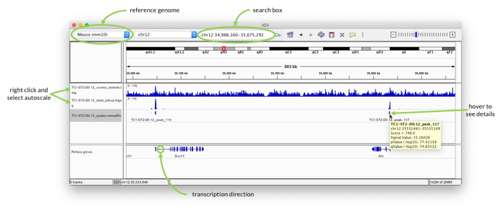
Start IGV and select mouse mm10 as genome in the drop-down menu in the upper left. Go to “File” -> “Load from File…” and select all three files in the output folder.
In the search box enter for example “Ahr” to check the signal around one of the genes highlighted in the paper.
Pay attention to the scale on which the two coverage tracks are shown. You can right-click on the track name on the left and select “Autoscale” to adjust the range.
When you hover over the blocks in the TC1-ST2-D0.12_peaks.narrowPeak track, you can see additional information about the called peaks, e.g. p-value. The peaks should be at the transcription start sites, because that is what H3K4me3 marks. Pay attention to the arrows in the “Refseq genes” track to see in which direction transcription goes.
Exercises#
You can find some exercises for this tutorial here.
(Optional) Revert the changes to your environment#
If you want to stop conda from always being active:
(access)$> conda init --reverseIn case you want to get rid of conda completely, you can now also delete the directory where you installed it (default is $HOME/miniconda3).
Useful stuff#
- If
PYTHONNOUSERSITEis set, Python won’t add theuser site-packages directorytosys.path. If it’s not set, Python will pick up packages from the user site-packages before packages from conda environments. This can lead to errors if package versions are incompatible and you cannot be sure anymore which version of a software/package you are using.
References#
- Köster, Johannes and Rahmann, Sven. “Snakemake - A scalable bioinformatics workflow engine”. Bioinformatics 2012.
- Gérard D, Schmidt F, Ginolhac A, Schmitz M, Halder R, Ebert P, Schulz MH, Sauter T, Sinkkonen L. Temporal enhancer profiling of parallel lineages identifies AHR and GLIS1 as regulators of mesenchymal multipotency. Nucleic Acids Research, Volume 47, Issue 3, 20 February 2019, Pages 1141–1163, https://doi.org/10.1093/nar/gky1240
- Langmead B, Salzberg S. Fast gapped-read alignment with Bowtie 2. Nature Methods. 2012, 9:357-359.
- Zhang et al. Model-based Analysis of ChIP-Seq (MACS). Genome Biol (2008) vol. 9 (9) pp. R137
Acknowledgements#
Many thanks to Aurélien Ginolhac, Cedric Laczny, Nikola de Lange and Roland Krause for their help in developing this tutorial.